3 Crosstabs and Two Independent Samples T-test (Week 15)
Data: Dell.sav
- Data is available on Moodle
3.1 Learning objectives
The aim of this third lab is to help you to use SPSS to examine group differences based on demographic factors. In this lab we will cover:
Chi-square test
The two independent samples t test
3.2 Chi-square Test
The chi-square test is useful for determining if differences exist between two categorical variables. This test can be used to substantiate perceived associations when calculating crosstabs such as those that you did in lab 1. Let’s say that you want to explore if there is an association between gender (Q14_gender) and number of hours spent on internet (Q1_online). A chi-square test would be useful to assess this.
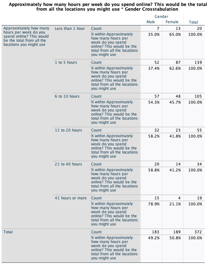
As in lab 1, use the menu options Analyze\(\rightarrow\)Descriptive statistics\(\rightarrow\)Crosstabs. I prefer to insert q14_gender into column and q1_online into row window–this way, you will see the distribution of gender within each category of q1_online. Select the statistics tab and click on the Chi-square option. Note that you can also click on Phi and Cramer’s V to get an indication of the strength of the association.
Using the cells tab you should also select row or column percents to help you to see the pattern of association (in this example, I prefer to select row percentages)
In the output window you will see that three (or four with the addition Phi and Cramer’s V) tables are produced. You can ignore the Case Processing Summary.
The second table is the crosstab table that you produced in lab 1 and the third table Chi-Square Tests gives you the new results. You will see that you have a table and graph like the one below for the gender by online crosstabs.
The p-value associated with the crosstabs is given by the following table
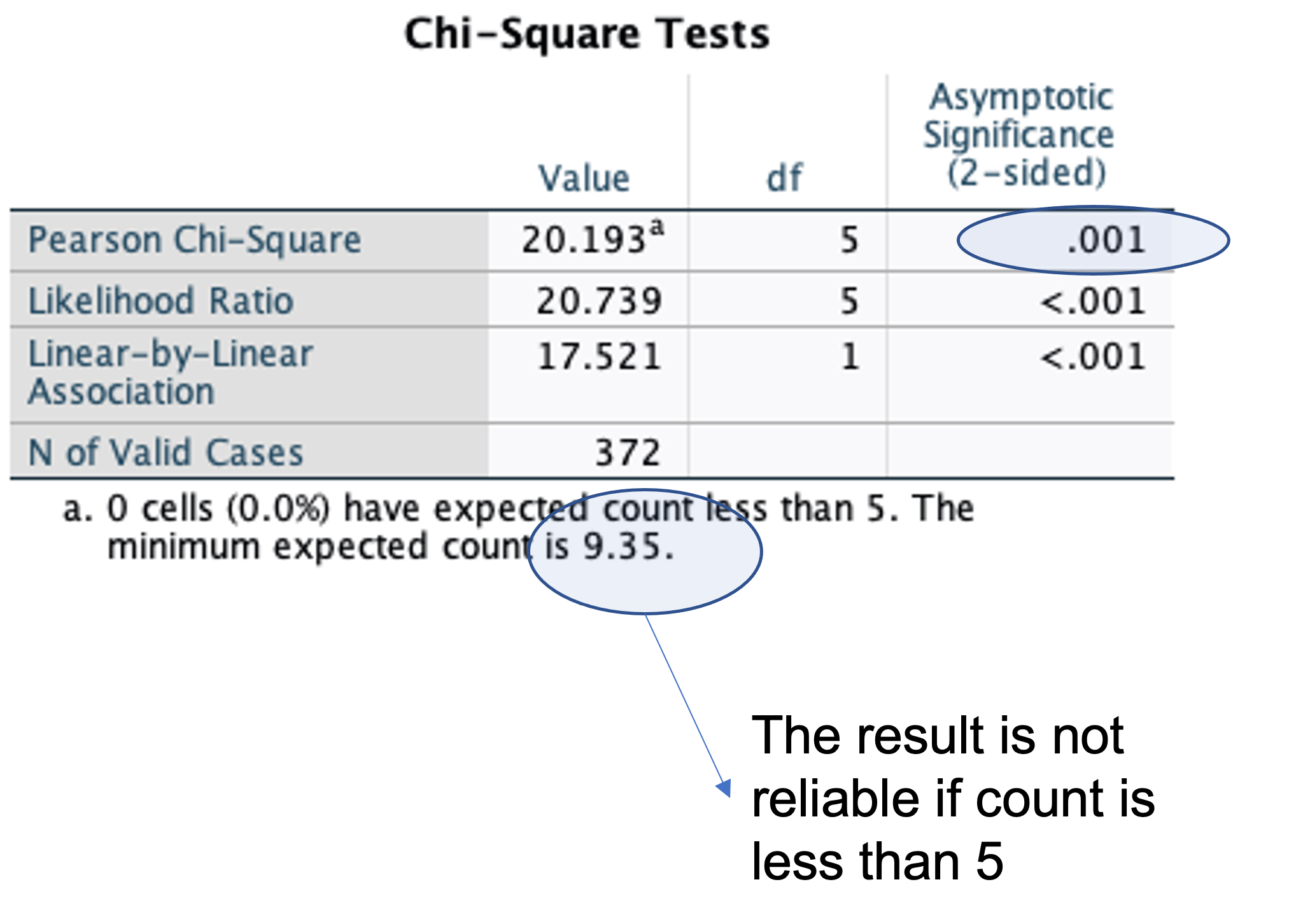
The most important column within the table is the “Asymp. Sig. (2-sided)”. This is the p-value column and the result above indicates that there is an evidence of an association between the rows and columns (because the p-value is smaller than 0.05), in this case between gender of the consumer and number of hours online. It is important to look at the proportion of consumers in each of the six groups.
If there was a statistically significant association you would ask the following:
Where do you see the association between the proportions of consumers?
How strong is the association?
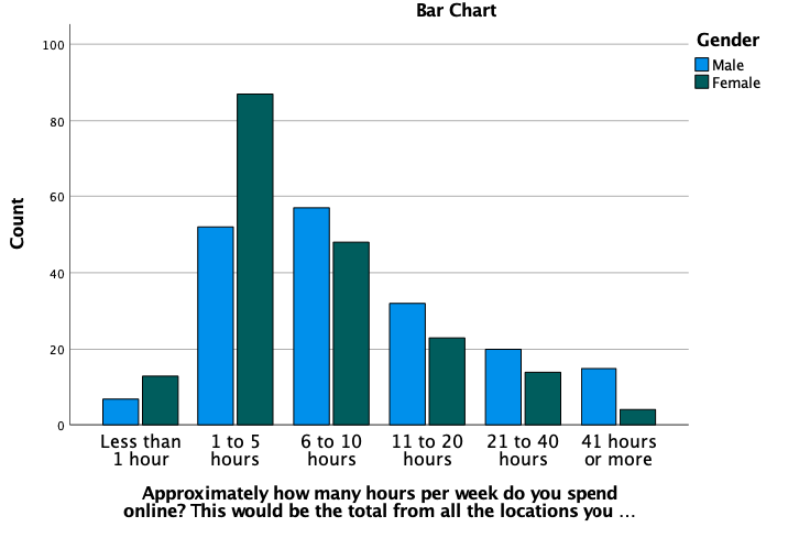
Have a look at the clustered bar chart, and explain the pattern of the association between hours spend online and gender. Is the association significant? (inspect the p-value of the Pearson Chi-Square)
Based on the Phi value, assess the strength the association between hours spend online and gender?
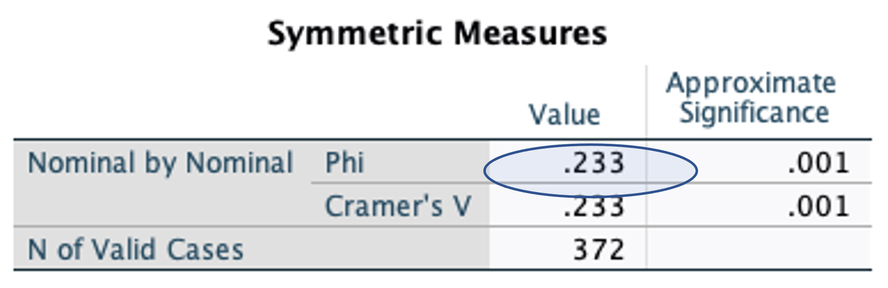
Phi tells us about the strength of an association. Its value ranges from 0 to 1. Cohen (1988) provides the following guideline:
0.1 is considered small
0.3 medium
0.5 large
3.2.1 Post-Hoc Test
If the association were significant, you would want to know further which group comparisons are actually significantly different. This is called post-hoc tests or multiple comparison tests. In essence, you want to test all pairwise comparisons to detect where the significant occurs. For example, is the proportion of male vs female significantly different within “less than 1-hour”, within “1-5 hours” group, etc?
How?
Use the menu options Analyze\(\rightarrow\)Descriptive statistics\(\rightarrow\)Crosstabs. Insert gender into “Columns” and q1_online into “rows”. Click Cells tab on the right, then TickRow percentages. Under z-test, tickCompare columns proportionsandAdjust p-values (Bonferroni method)`.
What does SPSS do with “Adjust p-values”? The answer is that SPSS will conduct z-tests for each comparison. Because of conducting multiple comparisons tests, the significance level at each test should not be 5% anymore. It should be divided by the number of comparisons. For example, if you have 6 pairwise comparisons, the sig. level at each test would be 0.05/6=0.008. This is to make sure that all comparisons tests were maintained at alpha=5%. If you do not adjust it and use alpha=5% in each of the pairwise tests, the probability of getting at least one significant result due to chance is high.
3.2.2 Post-Hoc Test Output
The output of the post-hoc test is given below
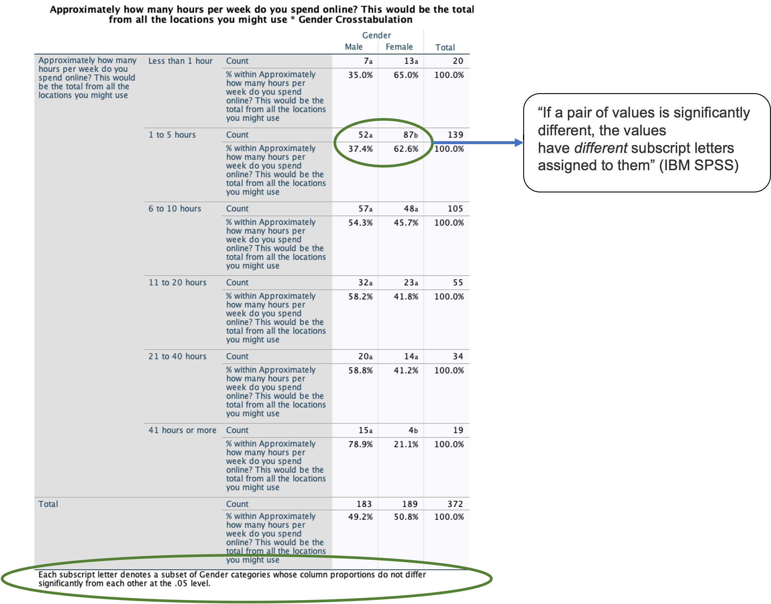
Looking at the output of the post-hoc test, what do you conclude?
3.3 Two Independent Samples T Test
This test allows you to explore differences in mean values across two groups e.g., between low vs. high-income groups; male vs. female consumers; those who received a reward vs. nothing; those who get a flu jab vs. placebo, country A vs. country B, etc.
Now, we want to assess if there are differences in the Opinion of Leadership (average scores of q10_op1, q10_op2, q10_op3) across gender (q14_gender).
As in the previous lab, you need to conduct reliability analysis to find out whether the three items of Opinion Leadership get well together, if yes, then you need to create a composite score by taking the average of the three items (I would suggest that you name the new variable as Opinion_avg).
In this lab, you will test following hypothesis:
H0: Opinion leadership of male consumers = Opinion leadership of female consumers.
H1: Opinion leadership of male consumers > Opinion leadership of female consumers.
The above alternative hypothesis is directional. Formulate a non-directional alternative hypothesis instead.
Note that when using a two independent samples test, the grouping variable (e.g., gender) is a qualitative variable – nominal or ordinal, and the test variable (e.g., amount money spent, scores on opinion leadership) is always a quantitative variable – interval or ratio.
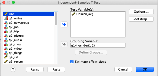
To conduct a T test, use the menu options Analyze\(\rightarrow\)Compare means\(\rightarrow\)Independent- Samples T test. The test variables will be Opinion_avg. The grouping variable is gender. You need to “define groups” this means telling SPSS that gender is measured using the numbers 1 and 2 (you will see from the data view that loyalty card status is coded as 1 and 2). By default, ‘Estimates effect size’ was ticked’.
3.3.1 Outputs
In the output window you will have three tables, the first giving the “Group Statistics”, the second giving the results of the “Independent Samples Test” (The important column is the sig. columns which give the p-values.), and the third gives the estimate of the effect size.
First, we need to look at the descriptive statistics to get a clear picture of the mean score of female vs. male on Opinion_avg, and assess the difference between the means.
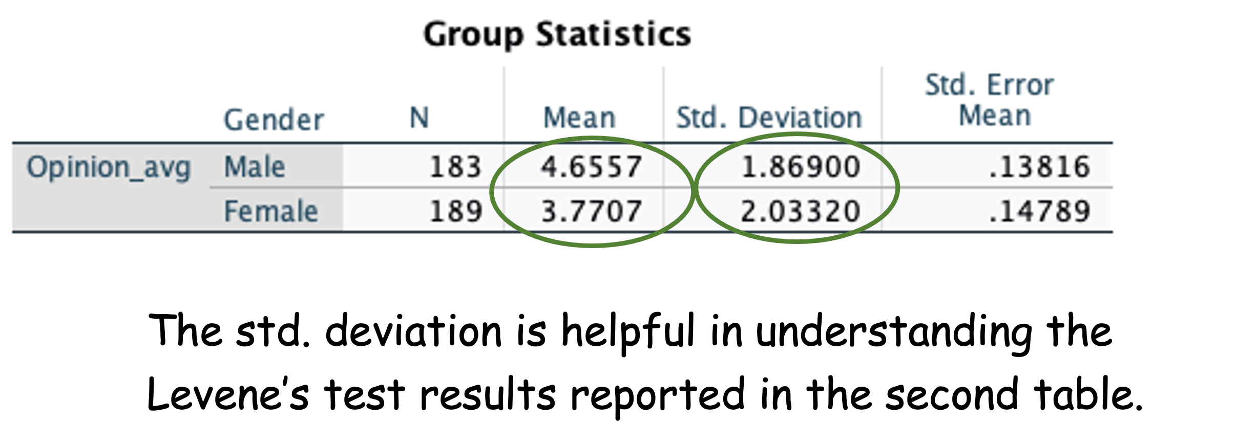
Look at the descriptive statistic above, say something about the mean scores and their standard deviations.
Now, let us discuss the second table.
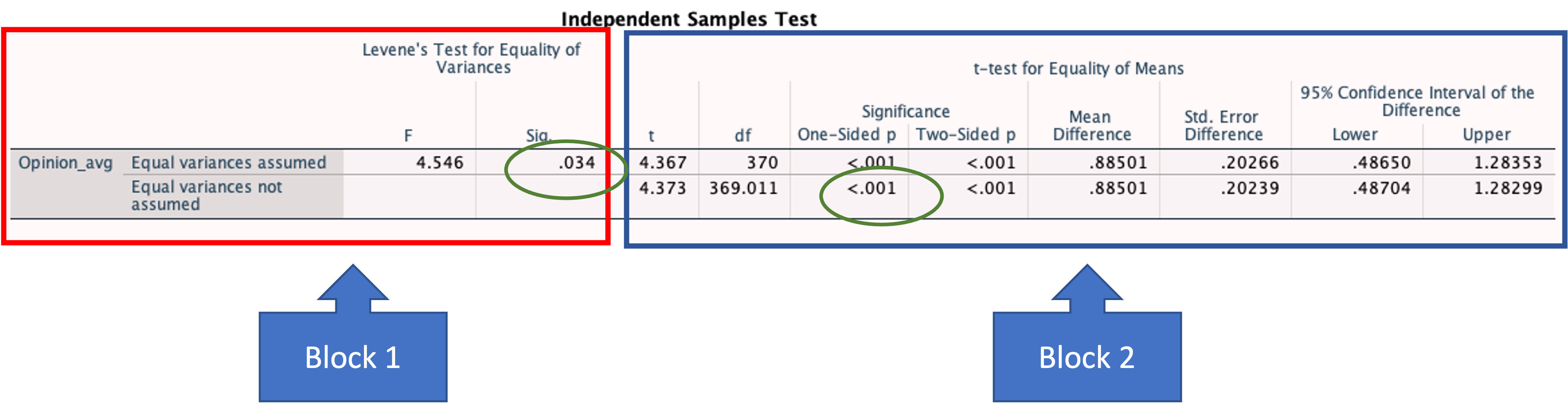
The second column in the table gives the significance value for Levene’s test (Block 1). This tells you if you can assume that the variance for the groups is equal, which cannot be assumed for this example and therefore when interpreting the result of the T-tests you should look at the p-value for “equal variances not assumed” (bottom row of Block 2). The p-value associated with the one-sided test was circled because our alternative hypothesis was directional (the males’ scores is higher than the females’ scores).
The one-sided p-value in the second block is significant (circled in green), what do you conclude?
3.3.2 Is the Difference Practically Meaningful?
If the mean difference is significant. We should ask if the different is meaningful or not. To answer this question, we need to assess the effect size table.
What is effect size? Imagine that if you took a paracetamol when you had a migraine and the pill reduces the pain slightly but it is not really helping you much – so the effect of the pill is small.
d = 0.2 is considered small
0.5 medium
0.8 large
For example, if the difference between two groups’ means < 0.2 standard deviations, despite the difference being significant, it is not practically meaningful.
Let us look at the effect size output below:
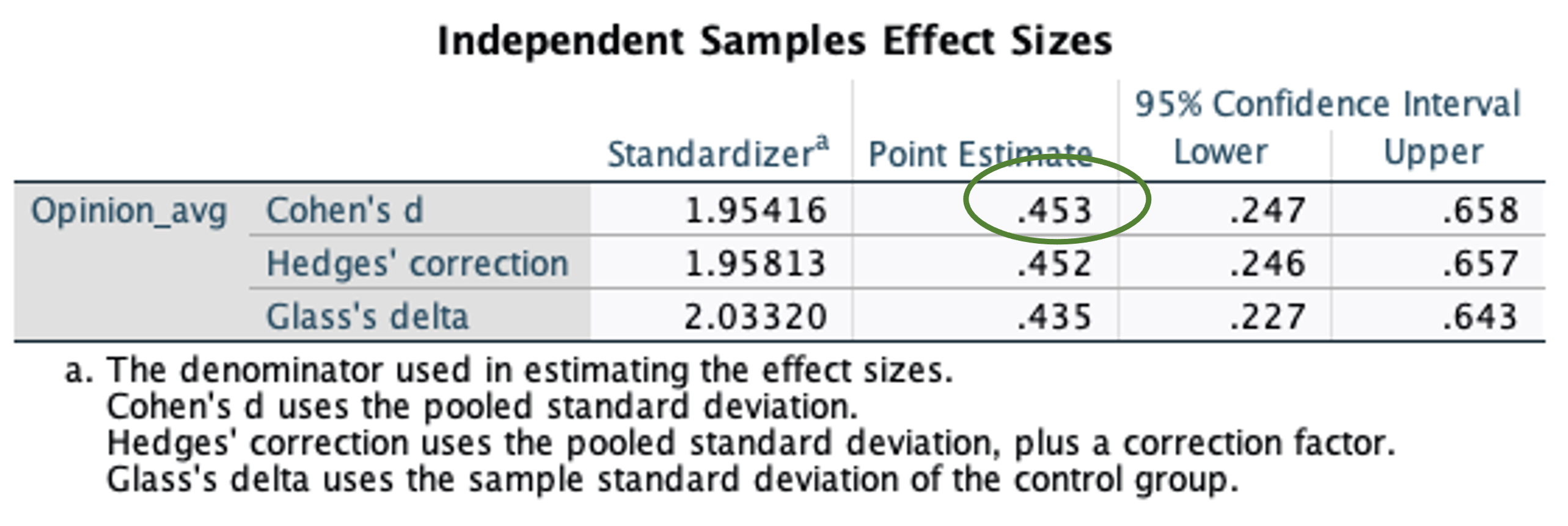
Look at the Cohen’s d in the above table, what does it tell you?
3.3.3 Interpretation of the Findings
Looking at the descriptive statistics and statistical results, we can conclude that there are statistically significant differences between male and female consumers on their ratings on opinion leadership. Specifically, male consumers have a higher rating of opinion leadership compared to that of female consumers (\(M_{Male} = 4.66\) vs. \(M_{Female} = 3.77\), Cohen’s d = 0.45). Furthermore in terms of the variability in the opinion leadership across the two groups (male and female consumers), the Levene’s test show that there are differences in the spread, that is, the variability in the opinion of leadership is not the same for both groups (\(SD_{Male} = 1.87\) vs. \(SD_{Female} = 2.03\)).
Why not investigating if there are differences in the satisfaction level between those who are willing to participate in Dell loyalty program and those who are not.
3.4 Video
3.5 Readings
Cohen, J. (1988). Statistical power analysis for the behavioral sciences, 2nd ed. Lawrence Erlbaum.
Feick, L. F., & Price, L. L. (1987). The market maven: A diffuser of marketplace information. Journal of Marketing, 51(1), 83-97.
Goldsmith, R. E., Flynn, L. R., & Goldsmith, E. B. (2003). Innovative consumers and market mavens. Journal of Marketing Theory and Practice, 11(4), 54-65.